DataScientist.blog

Welcome back to my Data Science blog, where we explore the fascinating world of data and its transformative power in the industry. Today, I want to dive into a crucial topic: Anomaly Detection. I’m currently working on a Predictive Maintenance (PM) project and have been researching the latest state-of-the-art algorithms for PM by reviewing numerous studies on the subject. In this post, I will introduce the most promising algorithms I’ve found.

Traditionally, anomaly detection in machinery relies on sensors such as vibration, acoustic, and current sensors. These sensors capture signals, which are then analyzed using techniques like Fourier transformation to identify anomalies. Another common technique is Wavelet transformation, which allows for the analysis of signals at multiple levels of resolution. But these are just a couple of the many techniques available. In this post, we’ll explore various methods used in anomaly detection.

While supervised learning methods are often employed, they require extensive datasets of abnormal conditions. However, anomalies are rare by nature, making it challenging to gather enough abnormal data for effective training. This is where the concept of a Digital Twin comes in handy. A Digital Twin is a virtual replica of a physical system that simulates real-world behavior and performance, providing valuable synthetic anomaly data for training. I find the Digital Twin technology very interesting and will certainly write about it another time, but due to time constraints, I won’t pursue it further in this project.

Another key point is the importance of dynamic learning in machine learning models. Unlike static rule-based systems, machine learning models can adapt to changing conditions by continuously learning and updating their understanding of what constitutes normal and abnormal behavior. In manufacturing, while production processes themselves may remain relatively constant, the condition of components can change significantly due to wear and tear. For example, when monitoring the condition of bearings, the wear progresses through four stages. Initially, when the bearing is new, it requires a run-in period, during which wear is relatively high until it settles in. In the second phase, the wear rate stabilizes and becomes minimal. In the third phase, wear starts to increase again. Finally, in the last phase, wear accelerates exponentially until failure. This is why it is crucial for a model to learn dynamically.

Despite the advancements in technology, accurately detecting anomalies remains challenging due to three main reasons: the sheer volume of data, the scarcity of anomaly data, and the complexity of patterns in time-series data, which is the focus of my project. In the upcoming sections, we’ll delve deeper into these challenges and discuss innovative solutions to overcome them.

Gaussian Mixture Model

When exploring anomaly detection, one can begin by diving into the data analysis process, which involves three main steps: preprocessing, modeling, and postprocessing.

First, in the preprocessing stage, sensor data is converted into a suitable format. This includes selecting the appropriate sensors, preparing the data, extracting relevant features, and choosing the condition states to monitor. For example, when dealing with machinery, one might opt for sensors that measure current because they are easier to install compared to vibration or acoustic sensors.

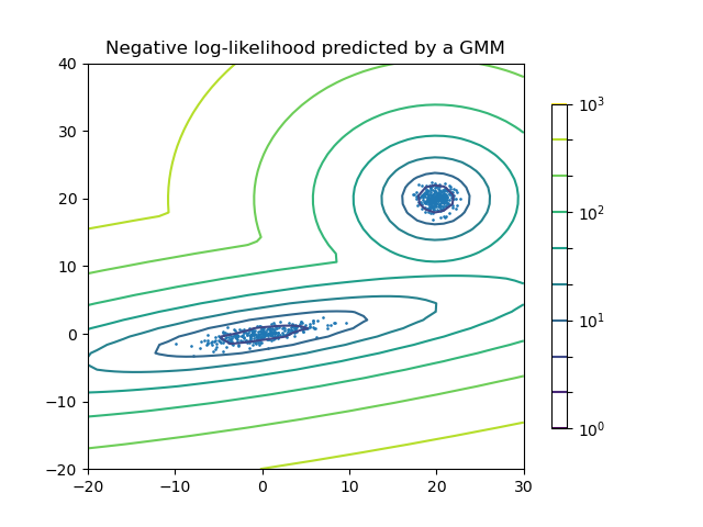
Next comes the modeling stage. One effective approach is using a Gaussian Mixture Model (GMM) for clustering the data to detect deviations from the normal state. A GMM is a probabilistic model that represents normally distributed subpopulations within an overall population. For instance, human height can be modeled with two normal distributions: one for males and one for females. GMMs are particularly useful because they handle uncertainties in cluster assignments and can model clusters of various shapes, not just circular ones. The beauty of this algorithm is that it does not assign a data point to a cluster rigidly but works with probabilities. For example, a data point can belong to Cluster A with 70% probability, Cluster B with 20%, and Cluster C with 10%.

The parameters of a GMM are estimated using the Expectation-Maximization (EM) algorithm, which iteratively performs two steps. The E-Step calculates the expected membership of each data point in each component, and the M-Step updates the parameters to maximize these expectations. This allows GMMs to provide a probabilistic description of the data distribution, making them more versatile than simpler clustering methods like k-means.

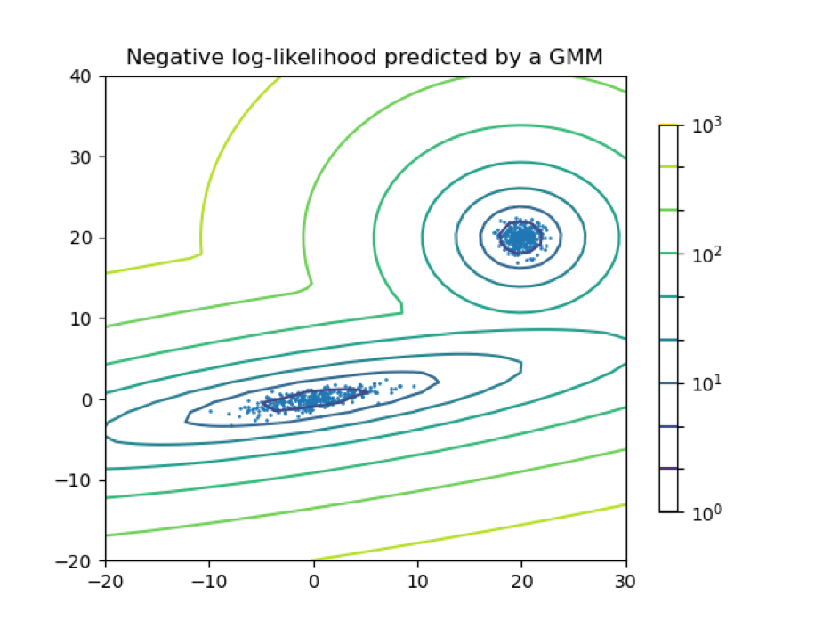
In the final stage, postprocessing, the anomalies are detected and quantified. The model calculates the probability that new data deviates from the learned normal states and compares this with a predefined threshold. [https://doi.org/10.1016/j.procir.2021.01.113]

Dynamic Time Warping and K-Means Clustering

Dynamic Time Warping (DTW) is a method for measuring similarity between two time series, even if they vary in length. Originally developed for speech recognition, DTW is now widely used for time series analysis.

In this study [https://doi.org/10.1016/j.procir.2023.09.146], DTW is combined with K-Means Clustering. K-Means is an unsupervised learning method that groups objects into clusters, ensuring objects within a cluster are more similar to each other than to those in other clusters. Here, K-Means with DTW is used to group screwing data and distinguish between normal (OK) and abnormal (not OK) processes.

Calculating DTW distances involves evaluating each pair of time series in the dataset to measure their similarity. This process creates a distance matrix where each entry (i,j) represents the DTW distance between the ith and jth time series. The DTW algorithm dynamically aligns the sequences to minimize their distance, accommodating variations in speed and timing. Once the DTW distances are calculated, a distance matrix is assembled from these values. This matrix serves as the input for the K-Means algorithm, replacing the traditional Euclidean distance.

Implementing K-Means clustering with the distance matrix begins by initializing k centroids, where k is the number of clusters to form. Each time series is assigned to the nearest centroid based on the DTW distance. The centroids are then recalculated as the mean of all time series in each cluster. This assignment step is repeated until convergence, ensuring that the clusters are optimized. To choose the optimal number of clusters, experiment with different values of k. In the study, various cluster numbers, ranging from 2 to 10, were tested. For each k, the K-Means algorithm is run multiple times to ensure robustness. The best configuration is selected based on evaluation metrics like accuracy or F1-Score, ensuring the most effective clustering of the time series data.

Isolation Forest

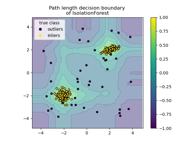
Isolation Forest is a method for outlier detection in high-dimensional datasets. It works by randomly selecting features and split values to isolate observations. Each observation’s path length, from root to leaf in the tree structure, is calculated. This method identifies anomalies because they tend to have shorter paths compared to normal observations.

Local Outlier Factor

The Local Outlier Factor (LOF) algorithm is an unsupervised method for detecting anomalies by evaluating the local density deviation of data points relative to their neighbors. LOF identifies outliers as samples with significantly lower density than their neighbors. The algorithm calculates a score reflecting the abnormality degree of each observation based on the ratio of the average local density of its k-nearest neighbors to its own local density. LOF is powerful because it considers both local and global dataset properties, performing well even when abnormal samples have different underlying densities.

DBSCAN

DBSCAN (Density-Based Spatial Clustering of Applications with Noise) is an unsupervised learning method used for clustering data points based on their density. It identifies clusters as dense regions in the data space separated by areas of lower density. This method is effective for detecting clusters of arbitrary shapes and handling noise and outliers, unlike other clustering methods like K-means, which work well for spherical clusters and are sensitive to noise. This capability is particularly valuable for sensor data, such as vibrations and acoustic sensors, which often come with significant noise.

Autoencoder

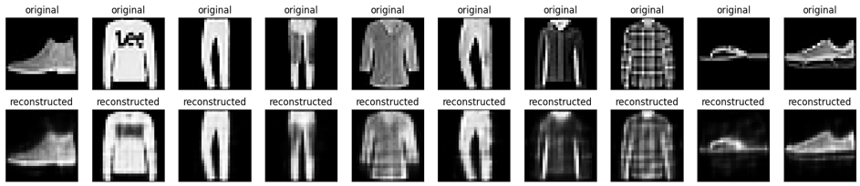
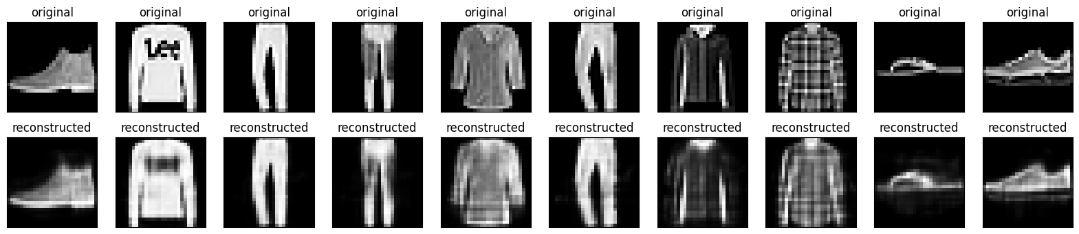
This is one of my favorites. An autoencoder is a special type of neural network that is trained to copy its input to its output. For example, given an image of a handwritten digit, an autoencoder first encodes the image into a lower dimensional latent representation, then decodes the latent representation back to an image. An autoencoder learns to compress the data while minimizing the reconstruction error.

One-Class SVM

One-Class Support Vector Machines (OCSVM) are a special type of Support Vector Machine designed for outlier, anomaly, or novelty detection. Unlike traditional SVMs used for classification, OCSVM identifies instances that deviate from the norm. It operates by defining a boundary around the normal data points, creating a region of normalcy. This boundary is crafted to maximize the margin around normal instances, enhancing the separation between normal and anomalous data. OCSVM finds applications in fraud detection, fault monitoring, network intrusion detection, and quality control in manufacturing (and maybe soon in predictive maintenance too ;).

In this study [https://doi.org/10.1016/j.cie.2023.109045], several models are tested for anomaly detection, including Isolation Forest (IF), Local Outlier Factor (LOF), DBSCAN, Autoencoder (AE), and One-Class SVM (OCSVM). The performance of these models is evaluated based on metrics such as precision, recall, and F1-score, as well as average computation time. The goal was to assess how well these models can identify faulty sensors.

In the results, the models IF, LOF, and DBSCAN demonstrate strong capabilities in anomaly detection, achieving high precision and recall values. The AE model shows high precision but has a lower recall rate, indicating a tendency towards false negatives. LOF, DBSCAN, and AE are effective at identifying the causes of faults, correctly identifying 9 faulty sensors each. However, OCSVM shows the highest number of false positives, making it less suitable for real-time fault detection.

Generally, one might accept false positive detections, as they indicate an anomaly was detected even when it wasn’t present—better to check too often than too little. This approach aligns with quality assurance practices, where over-inspection is preferable to under-inspection. However, in predictive maintenance, the situation is different. Maintenance personnel can quickly become dissatisfied if frequently tasked with unnecessary work. Therefore, in my project, it is particularly important to minimize false positive events to avoid burdening the maintenance team with redundant tasks. The authors of this study are my (unknown) colleagues, which is particularly advantageous because I can easily call them and delve deeper into the subject during a meeting.

Conclusion

In conclusion, while the reviewed studies provide a solid foundation, it is essential to recognize that their results may not directly translate to my specific project. Therefore, I plan to implement and test multiple algorithms to determine which ones work best for our unique conditions. By doing so, I can adapt these techniques to our data and operational requirements, ensuring the most effective anomaly detection and predictive maintenance outcomes. This approach will help fine-tune the models, addressing any challenges specific to our dataset and context, and ultimately optimizing our maintenance processes for better reliability and efficiency.